
Fuzzy Maps
EDIT Sep 2017 this post was written with a previous version of igraph that could read GML files produced by yEd.

Photo by WorldFish
It was in London at the Citizen Cyberscience Summit back in February 2014 that I first heard of Fuzzy Cognitive Maps or FCMs. I finally found some time to revisit the ideas behind FCM in more detail and experiment with free tools including yEd and igraph. Perhaps you’ll find the resulting script useful if you already use FCM in your work? Before going any further, let’s revisit briefly the idea behind shared mental models and why an FCM could help at all. Disclaimer: I am not an expert in FCMs or R. This post merely captures my tinkering and findings from various papers on this method. As we all know, making sense of the world that surrounds us is far from trivial. Luc de Brabandere in his MOOC on strategy reminded me that induction and deduction are two key mechanisms we use when we think about the external world. We use deduction when we apply mental models to the reality surrounding us. Induction is the reverse path where we start from reality and attempt mapping to some mental model. Induction is more challenging as it requires dealing with the extreme variety (i.e. states) found in real life. Over time, thinking becomes less about accumulating knowledge and more about devising actionable mental models through appropriate attenuation (i.e. forgetting, simplifying) of real-world variety. Robert Axelrod is credited with the use of so-called cognitive maps to show causal relationships among variables defined by non-experts. Nodes or vertices in the map represent concepts in a system or situation. Relation or edges represent cause and effect. These maps are directed graphs initially using only binary (+ or -) relationships. Kosko later introduced fuzzy logic to the approach allowing for relations to take values between -1 and +1. This range accomodates for nuances in language e.g. very high, high, medium, low, or very low effects.
Fuzzy Cognitive Maps
As societies structure themselves, sharing of mental models becomes increasingly important. They become the basis of norms and laws which will guide decision making. FCMs compete with other mental model approaches such as causal modeling, multi-attribute decision theory, or system dynamics. FCMs benefits include their ability to involve participants in building qualitative models: people quickly get that strengths and signs of connections represent how much one concept impacts the other. Ecologists are accustomed to dealing with mental models to try to understand environmental situations, e.g. managing fisheries. I am showing below an example taken from Oezesmi and Oezesmi.
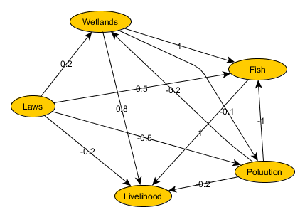
Download oezesmi.gml from GitHub
In the map above, weight -0.2 between pollution and wetlands indicates pollution is negatively affected by wetlands. Internally, the graph below is translated into a square adjacency matrix of weights where rows and columns correspond to concepts. Kosko was also the first to compute the outcome of an FCM as well as using them to evaluate different scenarios. The idea is to treat the map as a set of units of a neural network and apply an initial vector of size equal to the number of concepts in the map. The result is another vector of equal size (auto-associative neural network) which is re-submitted to the map until, hopefully, a stable state emerges. The initial vector reflects the state of affairs for a given scenario as defined by the modellers.
FCMs with R and yEd
There are tools out there to work with FCMs such as MentalModeler listed in the tools section of this blog or the Excel workbook from FCMappers. I was recently inspired by the release of an R package called FCMapper which motivated me to explore the use of R for FCM. As FCMs are digraphs, a handy tool that came to my mind is yEd. It allows me to quickly draw toy networks and experiment with common social network analysis (SNA) metrics. It even comes with fancy layout capabilities which are useful as you capture bigger models. When the SNA going gets tough, one indispensable R package is igraph which supports a wide range of graph models and associated metrics. As it is trivial to save models in yEd (in GML for my purpose) and load them into igraph, I figured I could implement my own set of routines to exploit FCMs using igraph from R.
The R script includes a number of functions to check a map captures with yEd, calculate concept-level and map-level indices, run baseline and alternative scenario calculations, visualize the impact of various scenarios and finally visualize the map with igraph (experimental and more for cross-check). It is possible to define a state vector corresponding to all concepts in the map and iteratively calculate the dot product of this state vector with the adjacency matrix of the map. An activation function is applied to this result. Typical functions include sigmoid, exponential or trivalent. This is captured in the central function below.
In addition to the initial state vector, a number of iterations to be reached before stopping, a vector of values to be pegged throughout iterations as well as a flag to run a transposed version of the dot product (to accomodate inconsistencies I found across FCM papers). Let’s show some examples.
I start capturing the model with yEd and save it as GML file. I then load the script from R and check the map to ensure I didn’t miss or mess up any weights on the edges. I imagine this is captured in lively sessions and typos or omission could easily occur. If all goes well, check.map() returns the graph object. I can then proceed to calculate indices related to the concepts in the map depicted above. Indices are computed against absolute values.
> source("fcm.R")
> check.map("oezesmi.gml")
IGRAPH D-W- 5 11 --
+ attr: id (v/n), label (v/c), graphics (v/c), LabelGraphics (v/c),
| label (e/c), graphics (e/c), LabelGraphics (e/c), weight (e/n)
+ edges:
[1] 5->1 3->1 1->2 5->2 1->3 3->4 2->4 1->4 5->4 5->3 3->2
> concept.indices("oezesmi.gml")
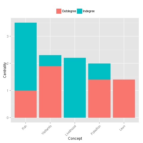
Concept Outdegree Indegree Centrality Transmitter Receiver Ordinary
1 Wetlands 1.9 0.4 2.3 FALSE FALSE TRUE
2 Fish 1.0 2.5 3.5 FALSE FALSE TRUE
3 Poluution 1.4 0.6 2.0 FALSE FALSE TRUE
4 Livelihood 0.0 2.2 2.2 FALSE TRUE FALSE
5 Laws 1.4 0.0 1.4 TRUE FALSE FALSE
Isolates
1 FALSE
2 FALSE
3 FALSE
4 FALSE
5 FALSE
>
Below is the graph generated for all concepts showing their cumulative, weighted, in- and out-degrees. The representation lets you quickly spot transmitter concepts which have positive outdegree and zero indegree. Such variables may benefit of a connection to self to prevent driving the state vector to zero throughout FCM iterations. This connection to self with weight 1 will be indicated when running check.map() as non-zero values on the adjacency matrix diagonal.
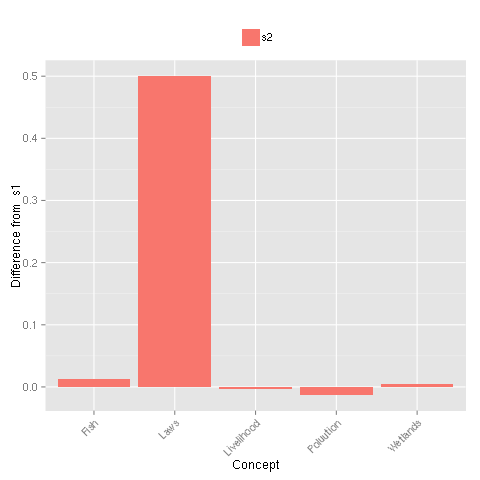
The snippet below shows how the script can be used to compare two scenarios using diff.scenarios(). In the paper, the authors explore the impact of completely eliminating domestic waste which results in highest reduction in lake pollution (row 3) and largest increase in lake protection regulation (row 5).
> s1<-baseline.scenario("oezesmi.gml",fn=fcm.sigmoid,lambda=0.2)
> s2<-alt.scenario("oezesmi.gml",peg=c(NA,NA,NA,NA,1),fn=fcm.sigmoid,lambda=0.2)
> diff.scenarios(s1,s2)
     Concept        s1        s2      Diff_s2     Chng_s2
1   Wetlands 0.5001500 0.5052748  0.005124828   1.0246582
2       Fish 0.5132542 0.5266135  0.013359289   2.6028601
3  Poluution 0.4850037 0.4725014 -0.012502348  -2.5777838
4 Livelihood 0.5357575 0.5317738 -0.003983746  -0.7435726
5       Laws 0.5000000 1.0000000  0.500000000 100.0000000
>
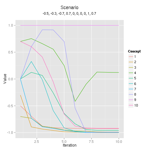
The iterations of FCM calculations are shown by the baseline.scenario() and alt.scenario() functions. In the example below from Szwed, I show an example of running a scenario for academic units focused on teaching (concept 4) from the paper. The intepretation of this scenario is that resulting values of the state vector show a decrease in teaching workload but also in students (concept 10).
> alt.scenario("szwed.gml",iter=10,trans=F,init=c(-0.5,-0.3,-0.7,0.7,0,0,0,0,1,0.7),peg=c(NA,NA,NA,NA,NA,NA,NA,NA,1,NA),fn=fcm.exp,lambda=2)
   Concept      Value
1        1 -0.9242856
2        2 -0.9976358
3        3 -0.9910089
4        4  0.1214240
5        5 -0.9587026
6        6 -0.9943509
7        7 -0.9969947
8        8 -0.9933041
9        9  1.0000000
10      10 -0.9202546
Warning message:
In alt.scenario("szwed.gml", iter = 10, trans = F, init = c(-0.5,  :
  Convergence not reached. Try increasing the number of iterations.

>
Download fcm.R from GitHub
Take Aways
Krystyna Stave of University of Nevada is a proponent of participatory modeling and systems thinking in environmental policy making. She designed a number of dashboards based on Vensim (a leading System Dynamics tool) to tackle water supply, minicpal waste, air quality or land use issues involving multiple stakeholders in participatory fashion. The SD approach requires some training though. FCM in contrast retains the visual approach, incorporates participation by design and doesn’t require sophisticated software. But FCMs are also sensitive to the way they are used and require an understanding of the state vector used, activation function and its parameters and the digraph itself. I thought it was simple enough to gain some insights and consider its use in the context of citizen sensing workshops where participants seek a systemic understanding of the data collected.
Sources
Gray, Gray, Cox, Henly-Shepard, Mental Modeler: A Fuzzy-Logic Cognitive Mapping Modeling Tool for Adaptive Environmental Management, 46th Hawaii Internation Conference on System Sciences, IEEE, pp. 965-973, 2013
Kok, The potential of Fuzzy Cognitive Maps for semi-quantitative scenario development, with an example from Brazil, Global Environmental Change, 19, pp. 122-133, 2009
Kosko, Fuzzy Cognitive Maps, International Journal of Man-Machine Studies, vol. 24, pp. 65-75, 1986
Oezesmi, Oezesmi, Ecological models based on people’s knowledge: a multi-step fuzzy cognitive mapping approach, Ecological Modelling, 176, pp. 43-64, 2004
Stave, Participatory System Dynamics Modeling for Sustainable Environmental Management: Observations from Four Cases, Sustainability, 2, pp. 2762-2784, 2010
Szwed, Application of Fuzzy Cognitive Maps to Analysis of Development Scenarios for Academic Units, Automatics, vol. 17, no. 2, pp. 229-239, 2013
 This material is licensed under CC BY 4.0